机器学习笔记（Chapter 05 - Logistic回归）

2016-02-09

Logistic回归根据现有数据对边界回归线建立回归公式，以此进行分类。训练分类器时的做法就是寻找最佳拟合参数，使用的是最优化算法。

Logistic回归和Sigmoid函数

Logistic回归过程
- 准备数据：需要进行距离运算，数据类型为数值型，结构化数据格式最佳。
- 分析数据：任意方法。
- 训练算法：大部分时间用于训练，训练目的为了找到最佳的分类回归系统。
- 测试算法：训练步骤完成后分类将会很快。
- 使用算法：输入数据并将其转换为对应的结构化数值，之后基于训练好的回归系数可以对这些数值进行简单的回归计算，判定其属于哪个类别。
Logistic回归优缺点
- 优点：计算代价不高，易于理解和实现
- 缺点：容易欠拟合，分类精度不高
- 使用数据类型：数值型和标称型
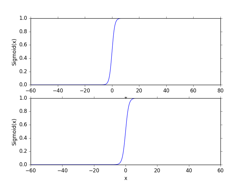
Sigmoid函数：是近似海维塞德阶跃函数（单位阶跃函数），σ(z)=1/(1+e^(-z))。当x为0时，Sigmoid(0)=0.5，随着x的增大减小，σ(x)将逼近1和0。当横坐标刻度足够大，Sigmoid看起来类似阶跃函数。我们将输入数据的每个特征乘以对应的回归系数，得到的结果相加，作为Sigmoid函数的参数，得到一个范围在0-1之间的数值，若大于0.5则归入1，小于0.5则归入0。因此Logistic回归可以被看成概率估计。

最佳回归系数确定

梯度上升法与梯度下降法类似，梯度上升算法用来求函数的最大值，梯度下降算法用来求函数的最小值。思想为要找到某函数的最大值，则沿着该函数的梯度方向探寻。梯度上升法到达每个点后会重新估计移动方向，循环迭代直至满足停止条件。对于线性回归系数，初始状态均为1，每次迭代的计算公式为w:=w+α▽f(w)，▽f(w)是在w处的梯度，α是沿梯度方向移动量大小，记为步长。该公式一直迭代执行，直到停止条件，比如迭代次数达到某个指定值，或误差达到指定精度。
使用梯度上升找到最佳参数，R为迭代次数，流程如下：
- 每个回归系数初始化为1
- 重复以下步骤R次：计算整个数据集的梯度，使用alpha*gradient更新回归系数的向量，返回回归系数
Code - gradAscent - logRegres.py

def sigmoid(inX):	# the array from numpy can be used as a single parameter
	return 1.0/(1+exp(-inX))
def gradAscent(dataMatIn, classLabels):
	dataMatrix = mat(dataMatIn)    # m*n
	labelMat = mat(classLabels).transpose()    # m*1
	m, n = shape(dataMatrix)
	alpha = 0.001
	maxCycles = 500
	weights = ones((n,1))    # n*1
	for k in range(maxCycles):
		h = sigmoid(dataMatrix*weights)	# m*1
		error = (labelMat - h)	# counting error direction, m*1
		weights = weights + alpha * dataMatrix.transpose() * error
	return weights

Code - loadDataSet - logRegres.py ，loadDataSet函数导入testSet.txt，返回数据矩阵和标签。gradAscent接收数据矩阵和标签，并返回生成的回归系数向量。

def loadDataSet():
	dataMat = []; labelMat = []
	fr = open('testSet.txt')
	for line in fr.readlines():
		lineArr = line.strip().split()
		dataMat.append([1.0, float(lineArr[0]), float(lineArr[1])])
		labelMat.append(int(lineArr[2]))
	return dataMat, labelMat

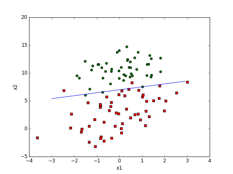
Code - plotBestFit - logRegres.py

def plotBestFit(weights):
	import matplotlib.pyplot as plt
	dataMat, labelMat = loadDataSet()
	dataArr = array(dataMat)
	n = shape(dataArr)[0]
	xcord1 = []; ycord1 = []
	xcord2 = []; ycord2 = []
	for i in range(n):
		if int(labelMat[i]) == 1:
			xcord1.append(dataArr[i,1]); ycord1.append(dataArr[i,2])
		else:
			xcord2.append(dataArr[i,1]); ycord2.append(dataArr[i,2])
	fig = plt.figure()
	ax = fig.add_subplot(111)
	ax.scatter(xcord1, ycord1, s = 30, c = 'red', marker = 's')
	ax.scatter(xcord2, ycord2, s = 30, c = 'green')
	x = arange(-3.0, 3.0, 0.1)
	y = (-weights[0]-weights[1]*x)/weights[2]
	ax.plot(x,y)
	plt.xlabel('x1'); plt.ylabel('x2');
	plt.show()

#>>> import logRegres
#>>> dataArr, labelMat = logRegres.loadDataSet()
#>>> weights = logRegres.gradAscent(dataArr, labelMat)
#>>> logRegres.plotBestFit(weights.getA())

随机梯度上升

gradAscent函数迭代五百次，并且每次计算都要遍历整个数据集，对于大规模数据复杂度过高。改进方法为每次仅用一个样本点来更新回归系数，只在新样本到来时对分类器进行增量式更新，是在线学习算法。流程如下。
- 所有回归系数初始化为1
- 对数据集中的每个样本：计算该样本的梯度，使用alpha*gradient更新回归系数值
- 返回回归系数值
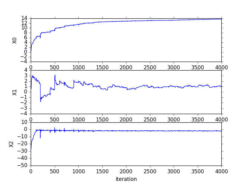
Code - stocGradAscent0 - logRegres.py，随机上升算法在200次迭代时的系数变化过程在《机器学习实战》82页，其中系数X2经过50次迭代后达到稳定，而系数1和0则需要更多次迭代。并且，在大的波动停止后，还有一些小的周期性波动，这源于数据中存在一些不能正确分类的样本点（数据集非线性可分），在每次迭代时会引发系统的剧烈震荡。

def stocGradAscent0(dataMatrix, classLabels):
	m, n = shape(dataMatrix)
	weights = ones(n)
	alpha = 0.01
	for i in range(m):
		h = sigmoid(sum(dataMatrix[i]*weights))
		error = classLabels[i] - h
		weights = weights + alpha * error * dataMatrix[i]
	return weights

Improve - Code -stocGradAscent1 - logRegres.py，改进后的代码中，alpha每次迭代都会调整，这可以缓解高频波动，并且虽然alpha随着迭代次数减小，但永远不会减小到0（常数项存在），这样保证多次迭代之后新数据仍然对系数有影响。同样，这也避免了alpha的严格下降，避免参数的严格下降也常见于模拟退火算法等其他优化算法中。改进后的代码通过随机选取样本的方式更新回归系数，这样可以减少周期性波动。改进后的代码收敛速度更快，默认迭代次数150。

def stocGradAscent1(dataMatrix, classLabels, numIter = 150):
	m, n = shape(dataMatrix)
	weights = ones(n)
	for j in range(numIter):
		dataIndex = range(m)
		for i in range(m):
			alpha = 4/(1.0+j+i)+0.0001
			randIndex = int(random.uniform(0, len(dataIndex)))
			h = sigmoid(sum(dataMatrix[randIndex]*weights))
			error = classLabels[randIndex] - h
			weights = weights + alpha * error * dataMatrix[randIndex]
			del(dataIndex[randIndex])
	return weights

改进后的回归系数

处理数据中的缺失值

假设有1000个样本和20个特征，若某传感器损坏导致一个特征无效，其余数据仍可用。
- 使用可用特征的均值填补缺失值
- 使用特殊值来填补确实值，如-1
- 忽略有缺失值的样本
- 使用相似样本的均值填补缺失值
- 使用另外的机器学习算法预测缺失值
对于Logistic回归，确实只用0代替可以保留现有数据，并且无需对算法进行修改。如果在测试数据集中发现某一条数据的类别标签已经缺失，Logistic回归的简单做法是将该数据丢弃，但如果采用类似kNN的方法则不太可行。
Code 用logistic回归从疝气病症预测病马死亡率 - logRegres.py

def classifyVector(inX, weights):
	prob = sigmoid(sum(inX*weights))
	if prob > 0.5 : return 1.0
	else: return 0.0

def colicTest():
	frTrain = open('horseColicTraining.txt')
	frTest = open('horseColicTest.txt')
	trainingSet = []; trainingLabels = []
	for line in frTrain.readlines():
		currLine = line.strip().split('\t')
		lineArr = []
		for i in range(21):
			lineArr.append(float(currLine[i]))
		trainingSet.append(lineArr)
		trainingLabels.append(float(currLine[21]))
	trainWeights = stocGradAscent1(array(trainingSet), trainingLabels, 1000)
	errorCount = 0; numTestVec = 0.0
	for line in frTest.readlines():
		numTestVec += 1.0
		currLine = line.strip().split('\t')
		lineArr = []
		for i  in range(21):
			lineArr.append(float(currLine[i]))
		if int(classifyVector(array(lineArr), trainWeights)) != int(currLine[21]) :
			errorCount += 1
	errorRate = (float(errorCount)/numTestVec)
	print "the error rate of this test is %f" % errorRate
	return errorRate

def multiTest():
	numTests = 10; errorSum = 0.0
	for k in range(numTests):
		errorSum += colicTest()
	print "after %d iterations the average error rate is: %f" % (numTests, errorSum/float(numTests))

Matplotlib绘制

备份下列几份代码（来自《机器学习实战》的github），大致了解matplotlib绘制的基本方法。

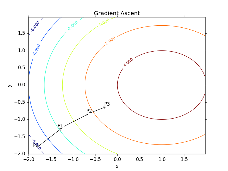
绘制等高线 - plotGD.py

import matplotlib
import numpy as np
import matplotlib.cm as cm
import matplotlib.mlab as mlab
import matplotlib.pyplot as plt

leafNode = dict(boxstyle="round4", fc="0.8")
arrow_args = dict(arrowstyle="<-")

matplotlib.rcParams['xtick.direction'] = 'out'
matplotlib.rcParams['ytick.direction'] = 'out'

delta = 0.025
x = np.arange(-2.0, 2.0, delta)
y = np.arange(-2.0, 2.0, delta)
X, Y = np.meshgrid(x, y)
Z1 = -((X-1)**2)
Z2 = -(Y**2)
#Z1 = mlab.bivariate_normal(X, Y, 1.0, 1.0, 0.0, 0.0)
#Z2 = mlab.bivariate_normal(X, Y, 1.5, 0.5, 1, 1)
# difference of Gaussians
Z = 1.0 * (Z2 + Z1)+5.0

# Create a simple contour plot with labels using default colors.  The
# inline argument to clabel will control whether the labels are draw
# over the line segments of the contour, removing the lines beneath
# the label
plt.figure()
CS = plt.contour(X, Y, Z)
plt.annotate('', xy=(0.05, 0.05),  xycoords='axes fraction',
             xytext=(0.2,0.2), textcoords='axes fraction',
             va="center", ha="center", bbox=leafNode, arrowprops=arrow_args )
plt.text(-1.9, -1.8, 'P0')
plt.annotate('', xy=(0.2,0.2),  xycoords='axes fraction',
             xytext=(0.35,0.3), textcoords='axes fraction',
             va="center", ha="center", bbox=leafNode, arrowprops=arrow_args )
plt.text(-1.35, -1.23, 'P1')
plt.annotate('', xy=(0.35,0.3),  xycoords='axes fraction',
             xytext=(0.45,0.35), textcoords='axes fraction',
             va="center", ha="center", bbox=leafNode, arrowprops=arrow_args )
plt.text(-0.7, -0.8, 'P2')
plt.text(-0.3, -0.6, 'P3')
plt.clabel(CS, inline=1, fontsize=10)
plt.title('Gradient Ascent')
plt.xlabel('x')
plt.ylabel('y')
plt.show()

生成图像如下
随机梯度上升过程中回归系数的变化 - plotGD.py

from numpy import *
import matplotlib
import matplotlib.pyplot as plt
from matplotlib.patches import Rectangle
import logRegres

def stocGradAscent0(dataMatrix, classLabels):
    m,n = shape(dataMatrix)
    alpha = 0.5
    weights = ones(n)   #initialize to all ones
    weightsHistory=zeros((500*m,n))
    for j in range(500):
        for i in range(m):
            h = logRegres.sigmoid(sum(dataMatrix[i]*weights))
            error = classLabels[i] - h
            weights = weights + alpha * error * dataMatrix[i]
            weightsHistory[j*m + i,:] = weights
    return weightsHistory

def stocGradAscent1(dataMatrix, classLabels):
    m,n = shape(dataMatrix)
    alpha = 0.4
    weights = ones(n)   #initialize to all ones
    weightsHistory=zeros((40*m,n))
    for j in range(40):
        dataIndex = range(m)
        for i in range(m):
            alpha = 4/(1.0+j+i)+0.01
            randIndex = int(random.uniform(0,len(dataIndex)))
            h = logRegres.sigmoid(sum(dataMatrix[randIndex]*weights))
            error = classLabels[randIndex] - h
            #print error
            weights = weights + alpha * error * dataMatrix[randIndex]
            weightsHistory[j*m + i,:] = weights
            del(dataIndex[randIndex])
    print weights
    return weightsHistory
    

dataMat,labelMat=logRegres.loadDataSet()
dataArr = array(dataMat)
myHist = stocGradAscent1(dataArr,labelMat)


n = shape(dataArr)[0] #number of points to create
xcord1 = []; ycord1 = []
xcord2 = []; ycord2 = []

markers =[]
colors =[]


fig = plt.figure()
ax = fig.add_subplot(311)    # take care
type1 = ax.plot(myHist[:,0])
plt.ylabel('X0')
ax = fig.add_subplot(312)
type1 = ax.plot(myHist[:,1])
plt.ylabel('X1')
ax = fig.add_subplot(313)
type1 = ax.plot(myHist[:,2])
plt.xlabel('iteration')
plt.ylabel('X2')
plt.show()

生成图像如下
生成sigmoid函数 - sigmoidPlot.py

import sys
from pylab import *

t = arange(-60.0, 60.3, 0.1)
s = 1/(1 + exp(-t))
ax = subplot(211)
ax.plot(t,s)
#ax.axis([-5,5,0,1])
plt.xlabel('x')
plt.ylabel('Sigmoid(x)')
ax = subplot(212)    # x-y-index
ax.plot(t,s)
ax.axis([-60,60,0,1])    # x-index width
plt.xlabel('x')
plt.ylabel('Sigmoid(x)')
show()

生成图像如下

Logistic回归总结

Logistic回归的目的是寻找一个非线性函数Sigmoid的最佳拟合参数，求解过程可以由最优化算法完成。随机梯度上升算法可以简化梯度上升算法，获取几乎相同的效果，并且占用更少的计算资源，在新数据到来时完成在线更新，而不需要重新读取整个数据集。

参考文献：《机器学习实战 - 美Peter Harrington》

原创作品，允许转载，转载时无需告知，但请务必以超链接形式标明文章原始出处(https://forec.github.io/2016/02/09/machinelearning5/) 、作者信息（Forec）和本声明。

大数据/分布式系统

Logistic回归和Sigmoid函数

最佳回归系数确定

随机梯度上升

处理数据中的缺失值

Matplotlib绘制

Logistic回归总结